Introduction:
Much like with schlieren, we are constantly confronted with the question of how we optically measure something that is invisible. With schlieren, we take advantage of the fact that density gradients actually do make themselves visible. With Particle Image Velocimetry (PIV), we take a different approach – if we can’t see the air, let’s put something in the air that we can see, and look at that instead.
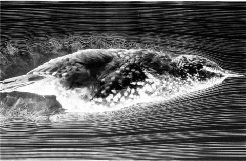
This approach has been used since the very beginning of fluid mechanics research – if you want to visualize flow patterns in air, fill the air with smoke and watch how the smoke moves. A beautiful example of this is presented in the image below: the flow around a flying starling visualized with smoke tracers.
How does it work?
Particle Image Velocimetry takes this approach one step further. Rather than just looking at the motion of the smoke, can we actually track the motion of individual smoke particles? (note: smoke is just one example of a tracer, in water we use hollow glass beads, there are many other options). If we illuminate our particles with a laser pulse of very short duration (typically on the order of 10 nanoseconds or less), we can take a photo with the motion of those particles “frozen” at an instant time.
In our supersonic jet, that might look something like this:
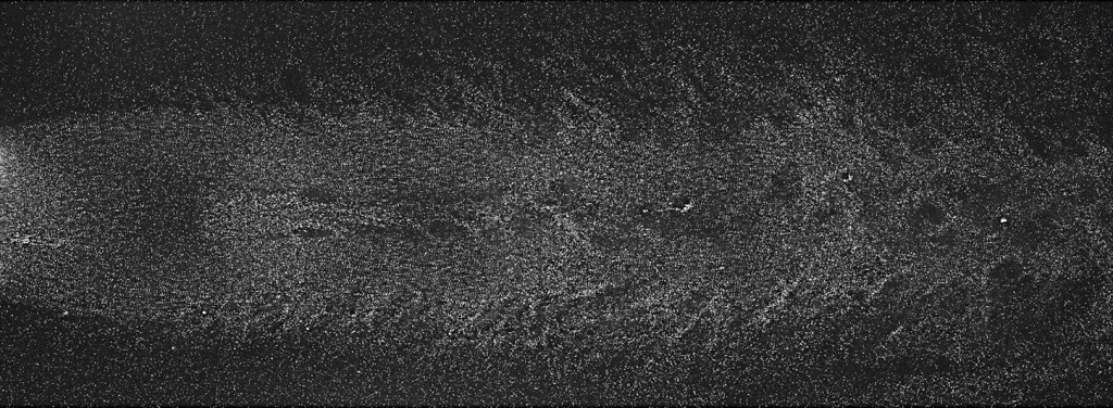
We see a whole field of particles, and we can see some of the structures in the jet, but this alone doesn’t really tell us anything extra.
The trick is to take not one photograph, but two. Using specialized cameras, we take two photographs with only a short time separation between them. If we are studying a relatively slow flow, the gap between the two photographs might be a few milliseconds. For really fast flows (like the supersonic jets we study), there is usually only a few hundred nanoseconds between the photographs. That’s really fast! To do this of course, we also need a laser that can fire two really bright pulses of light in very quick succession – we use a “dual-cavity” laser to achieve this.
Once we have the two photos, we start to get some idea of the motion in the flow. It might look something like this:
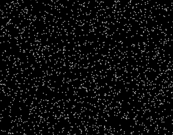
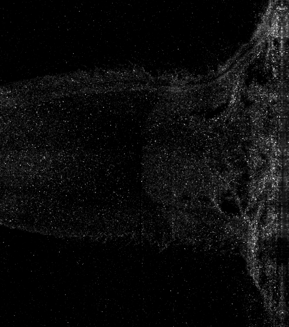
This is a synthetic image where every particle moves the same amount. Figuring out how things are moving from this is probably pretty straightforward. In a real flow of course, the motion is much more complicated:
To get really useful information out of this though, we need to be able to extract flow velocities from it. We do this by dividing the image up into a whole lot of small regions, called interrogation windows. As an example, we might divide up our image something like this:
Now we will apply a mathematical technique called “cross correlation” to each of these small boxes – the interrogation windows. How does that work?
Let’s imagine we look at one of our little windows here, and we see three particle images there (in practice we’d usually want to see at least 10, but that gets hard to draw!)
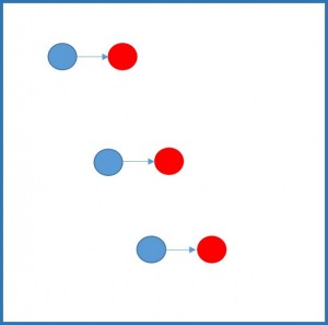
Let’s imagine in the first photo we took, we see the blue particles, in the second photo we took, we see the red particles. We of course don’t get to see the arrows, but for this example, they’re there to tell us all three of the particles have moved by the same amount. We can tell just by looking at it that these particles have moved the same amount, but looking by eye isn’t much use when we need to process thousands of these windows, in thousands of different images! We need a way to do it mathematically. This is where the cross correlation comes in.
We can tell which blue particle corresponds to which red particle, if we assume they’re all moving the same amount. But if we don’t know in advance how the flow is moving, we can’t actually say for sure which blue particle matches which red one. With cross correlation, we do this on a statistical basis. As an example, let’s consider each of the blue particles in turn.
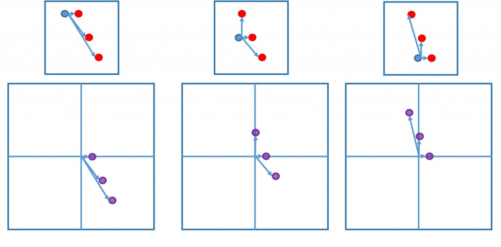
In the first frame of the figure here, we consider the uppermost blue particle. We consider the possibility that it corresponds to each of the red particles. On the grid below, we indicate each of these possibilities based on the displacement the particle would have to have experienced relative to its initial position. We then repeat the process for the middle and lower particles, as indicated.
If we then add these correlation maps together, we might get something that looks like this:
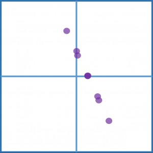
These dots represent all the possible displacements of particles within the window. If you look carefully though, you’ll see that one dot is much darker than the rest – it’s actually three dots superimposed on each other! That’s because when we correctly matched each blue particle with the appropriate red particle, they all had displaced by the same amount. When we consider all three particles, the dot corresponding to the “true” displacement shows up three times, the rest only show up once each. These dots add together to form a peak on our correlation plane.
You can imagine if we have more particles, the effect is even stronger – it gets easier to pick out the true displacement. Once we have an estimate of the displacement, since we also know the time between our two photos, we can now calculate the velocity (velocity is displacement divided by time). If we do this for every window in our image, we now have a map of how the velocity varies in the flow.
We have calculated the velocity by looking at images of particles. This is where the technique derives its name: Particle Image Velocimetry.
Of course, this all assumes that the particles are moving at the same speed as the fluid. For small particles and slow flows this is typically a safe assumption. Once compressibility effects become important and shockwaves form in the flow, this can be a lot harder to achieve. See my paper in Experiments in Fluids for more details.
Some applications:
Particle Image Velocity is now the gold-standard technique for velocity measurement in fluids. It is used to study everything from aerodynamics to biological systems, fundamental turbulence to combustion.
This stunning video from the University of Brighton shows PIV being performed inside the cylinder of an optical engine.
In our own laboratory we use PIV to study a whole range of flows: supersonic jets, turbulent boundary layers, pharmaceutical flows, and a whole range of others. We develop the majority of our own systems in-house, and have been doing so since Prof. Julio Soria first wrote his own PIV code over twenty years ago. More recently, Dr. Callum Atkinson produced some of the seminal work on tomographic PIV – a technique that allows us to measure a whole three dimensional field instead of just a slice. Check out the Research page to see some of the projects we are applying PIV to.