Hydrodynamic stability, that is the tendency of infinitesimal perturbations to fluid mechanical systems to grow in amplitude, has been studied since the nineteenth century. Amongst the best known early experimental examples comes from the work of Osborne Reynolds, whose sketches of pipe flow are shown below:
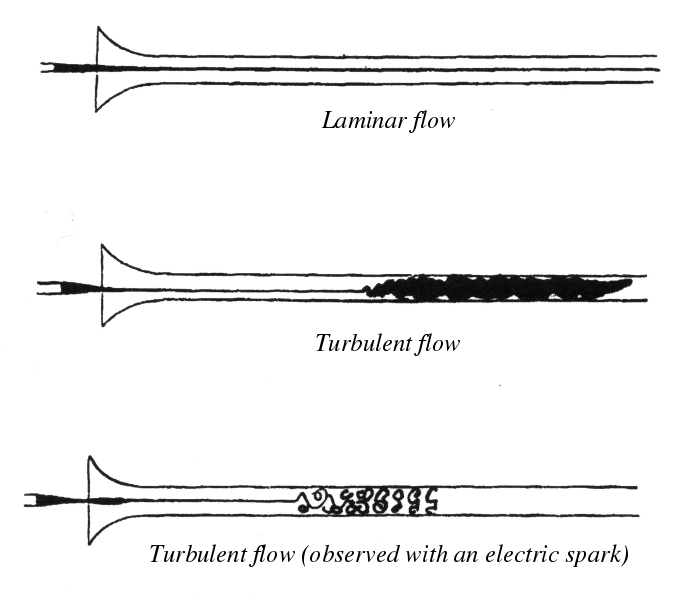
Sketches of laminar and turbulent flow in a pipe, Reynolds (1883).
Reynolds demonstrated that at sufficiently low speeds, the dye he injected into the pipe “extended in a beautiful straight line through the tube”. As the flow velocity increased, the line of dye would begin to shift around, and then with further increases, some critical velocity would be reached where the dye would begin to mix with the surrounding water. When the flow was observed with a spark (to freeze the motion at a moment in time), this mixing was observed to be characterized by “a mass of more or less distinct curls, showing eddies.”
Reynolds’ experiments have been duplicated thousands of times over, but a particularly beautiful example of this transition process (though different to the pipe flow experiment of Reynolds) can be seen in the following video:
There are many forms of hydrodynamic instability, driven by buoyancy, shear, surface tension, centrifugal force, and various other mechanisms that may disturb the equilibrium between the forces acting on the fluid and its internal dissipative mechanisms. In our consideration of jet noise however, there is one mechanism of hydrodynamic instability that concerns us above all others, and that is the Kelvin-Helmholtz instability, beautifully visualized in the video below:
Our goal here is thus to furnish ourselves with the tools to understand what the Kelvin-Helmholtz instability is, and to predict when and where it will occur. For a further introductory explanation of the Kelvin-Helmholtz instability, the same Youtube Channel as above, Sixty Symbols, has an interview with Prof. Mike Merryfield from the University of Nottingham, who provides an excellent discussion in lay language as to how the structures associated with the KH instability form.
So, we know what the Kelvin-Helmholtz instability looks like, and we have a sort of lay-appropriate explanation for how it works, but can we predict it mathematically? We certainly can, head on over and see the most simplified form of the KH problem explored:
An Introduction to the Mathematics Underpinning the Kelvin-Helmholtz Instability In a Simple Mixing Layer
So, now you know a little bit about the Kelvin-Helmholtz instability, at least how it works in a very idealized system where we ignored most of the real physics. In a real flow, where we have compressibility, viscosity, and a continuous velocity profile rather than a discontinuity it….. actually works in qualitatively the same way, and we can even get fairly reasonable estimates of which frequencies will be the most unstable in a real flow from the very simplified analysis that we considered above. It’s not perfect, but it’s a start. If we want to do more complex mathematics, we can of course get much closer. We’ll come back to that later.
For now, let’s get back to our discussion of jets.
What about if we wanted to look at a vortex-sheet solution for a jet instead of a mixing layer, and include compressibility?