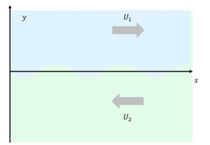
We will now explore a mathematical demonstration of the Kelvin-Helmholtz instability in its most basic form. Let’s begin by considering the simple flow schematic shown below, two horizontal, parallel, infinite streams of fluid, each uniformly moving in opposite directions; fluid one is blue, fluid two is green. In a fuller description of the KH instability, we could consider the fluids as being of different densities, but we are going to keep things extremely simple here, and imagine both streams are of the same density, and the only difference is in the velocity. The line dividing these two fluids can be considered to be a “vortex sheet“, as it is a discontinuity in the fluid velocity.

Our task is now to consider the stability of this very simple system. For our purposes here, we will consider the most basic possible analysis, which is to assume that the fluid is both inviscid and incompressible. The analysis we are going to conduct, is to consider the equations of motion that describe this system, we will then linearize the system, and consider the response of this linear system to infinitely small perturbations; if the system grows in response to an infinitely small perturbation, it is unstable. To determine if this system is stable, we will undertake the following steps:
- Establish the equations of motion.
- Linearize these equations of motion.
- Propose an ansatz (a model solution) and substitute it into our linearized equations
- Obtain an ordinary differential equation from re-arranging our linearized equations
- Impose appropriate boundary conditions to reframe the problem as an eigenvalue problem
- Solve the eigenvalue problem to determine the stability of the system
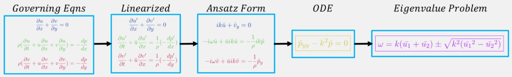
To signpost what we’ll be doing, here it is represented diagramatically.
Establish the equations of motion.
The governing equations of motion for fluids are the conservation of mass, momentum, and energy. At this early stage we can omit the conservation of energy statement, as our assumption of incompressibility means we don’t need it to form a solution. We will also remove a number of terms by assuming that the flow is inviscid and two-dimensional. For compactness, we will write our initial conservation statements using vector notation, we could make this more compact still using tensor notation, but as that is unfamiliar to many people when starting out, we’ll stick with vector form. If you are unfamiliar with the vector form, click the little “expand” option to see them in standard differential form.
We are going to rework these equations into a number of different forms, so to help keep track of them, I will colour code them. When we arrive at key results with these equations in different form, I will use the same colours.
Conservation of Mass in Vector Form (2D, Incompressible)
![\[ \centering \nabla \cdot\mathbf{u} = 0 \]](https://daniel.edgington-mitchell.com/wp-content/ql-cache/quicklatex.com-6ddb6a3106f682a16b4da85ec4bc53e7_l3.png "Rendered by QuickLaTeX.com")
![\[ \centering \frac {\partial u} {\partial x} + \frac{\partial v}{\partial y} = 0 \]](https://daniel.edgington-mitchell.com/wp-content/ql-cache/quicklatex.com-afb6e00cfcc865fc0687b23eb1b524ca_l3.png "Rendered by QuickLaTeX.com")
Conservation of X-Momentum in Vector Form (2D, Incompressible, Inviscid)
![\[ \centering \rho ( \frac{\partial u}{\partial t}+\nabla u \cdot \mathbf{u})=-\frac{dp}{dx} \]](https://daniel.edgington-mitchell.com/wp-content/ql-cache/quicklatex.com-13cc77aa90f36e2916a9a86491d339b4_l3.png "Rendered by QuickLaTeX.com")
![\[ \centering \rho ( \frac{\partial u}{\partial t}+ u \frac{\partial u}{\partial x} + v \frac{\partial u}{\partial y}) =-\frac{dp}{dx} \]](https://daniel.edgington-mitchell.com/wp-content/ql-cache/quicklatex.com-b3002632a64ba16a095961bd7deed845_l3.png "Rendered by QuickLaTeX.com")
Conservation of Y-Momentum in Vector Form (2D, Incompressible, Inviscid)
![\[ \centering \rho ( \frac{\partial v}{\partial t}+\nabla v \cdot \mathbf{u} )=-\frac{dp}{dy} \]](https://daniel.edgington-mitchell.com/wp-content/ql-cache/quicklatex.com-9b3deb5828cbaae9ebbf2acb38226e4e_l3.png "Rendered by QuickLaTeX.com")
![\[ \centering \rho ( \frac{\partial v}{\partial t}+ u\frac{\partial v}{\partial x} + v \frac{\partial v}{\partial y}) =-\frac{dp}{dy} \]](https://daniel.edgington-mitchell.com/wp-content/ql-cache/quicklatex.com-4b457f4a371cf25c6d7ce9ec0c70d03f_l3.png "Rendered by QuickLaTeX.com")
Here  and
and  are our velocity components in the
  and
and  direction, and
  is a vector of these velocities
 ![\mathbf{u}=[u,v]](https://daniel.edgington-mitchell.com/wp-content/ql-cache/quicklatex.com-451cf6e73734250af2e953c4e107d1e1_l3.png "Rendered by QuickLaTeX.com") .
.
And that’s it, these are our equations of motion!
Linearize the equations of motion.
As a first step towards linearization, we now apply the Reynolds Decomposition to these equations, meaning we decompose all variables (![q=[u,v,p]](https://daniel.edgington-mitchell.com/wp-content/ql-cache/quicklatex.com-91b1d0f87a6718ed9f661c5c51d1e680_l3.png "Rendered by QuickLaTeX.com") ) into a temporal mean
) into a temporal mean  and fluctuating
  component.

First, we apply this to the continuity equation:
Conservation of Mass – Reynolds Decomposition

When we are not used to manipulating these equations, it is easiest to expand this into its full form:

We then substitute in our Reynolds-decomposed variables:

Now, to simplify this further, we consider our initial problem description, which is that we have two infinite parallel streams, each uniform within its region..
- If the flows are parallel, they can have no vertical velocity component, so
 .
. - Since each flow is uniform within its region, they can have no velocity gradient in x, so

Thus our equation reduces to:
![\[ \centering \boxed{\frac {\partial u'} {\partial x} + \frac{\partial v'}{\partial y} = 0} \]](https://daniel.edgington-mitchell.com/wp-content/ql-cache/quicklatex.com-a911c9546680bd49924cd0af48e8f57e_l3.png "Rendered by QuickLaTeX.com")
Conservation of x-momentum – Reynolds Decomposition
We now apply the same decomposition to the x-momentum equation. The decomposition for the time derivative and pressure gradient are straightforward, so these can be done first:

Becomes:

Now, we expand the term  and perform our Reynolds decomposition and substitution:

And now substitute, using the product rule:

Now, if we were to substitute these two into our x-momentum equation, we would end up with an additional 8 terms, which is going to end up with a very small fontsize if we want to fit it on one page. Luckily, there are two steps we can take to simplify here. The first is a repeat of the simplifications made when considering the continuity equation: our flows are parallel and infinite, and uniform within their region. Thus once again,  . Once these terms are set to zero, our eight terms reduce to three:

At this stage of a section called “linearization”, we have not yet actually linearized anything! We now introduce our first linearizing assumption: our fluctuations are small relative to our mean, sufficiently small that the product of fluctuations can be neglected. In the above equation, two of our three terms appear to involve products of fluctuations ( ). However, strictly speaking, these are actually the products of fluctuations and the derivative of fluctuations, which is not quite the same thing; even if the fluctuations are small, their derivatives may not be. However, we can perform a little re-arrangement to get the result we need:
Let’s start with something that we know is equal to zero, i.e. the product of two fluctuations  . If we take the divergence of this product:

We have already shown from continuity that  , and the term
  on the LHS is the product of two fluctuations, so is also assumed to be zero under our linear approximation, therefore
  , demonstrating in this case the products of the fluctuating components with their derivatives are also zero.
We set to zero, and are left only with a single term:

Thus our original equation becomes:

We remove a few remaining terms by considering that the temporal mean of a time derivative must be zero by definition, so  , and under the assumptions of inviscid, infinite, uniform flow, there can be no mean pressure gradient:
  .
.
It is worth noting at this point that we are removing these terms based on arguments that are intended to be more intuitive than rigorous. Later, when we revisit stability analysis for flows with less simplifying assumptions, we will be more rigorous in our justification for how these equations are simplified.
Thus concludes our substitution of the Reynolds decomposition, and our linearization of the x-momentum equation:
![\[ \centering \boxed{\frac{\partial u'}{\partial t}+\bar{u}\frac{\partial{u'}}{\partial x}=\frac{1}{\rho}(-\frac{dp'}{dx})} \]](https://daniel.edgington-mitchell.com/wp-content/ql-cache/quicklatex.com-d98e024c6cf70ad62115e3d132c51c5c_l3.png "Rendered by QuickLaTeX.com")
Conservation of y-momentum – Reynolds Decomposition
The procedure for the y-momentum linearization is identical to the x-momentum equation, so you can click here to see a few intermediate steps, or just skip straight to the result:


![\[ \centering \boxed{\frac{\partial v'}{\partial t}+\bar{u}\frac{\partial{v'}}{\partial x}=\frac{1}{\rho}(-\frac{dp'}{dy})} \]](https://daniel.edgington-mitchell.com/wp-content/ql-cache/quicklatex.com-12fb3b4241952e709daf4e0b66ff82a0_l3.png "Rendered by QuickLaTeX.com")
Linearized Incompressible Inviscid 2D Equations of Motion
Try saying that three times fast. Here they are:
![\[ \frac {\partial u'} {\partial x} + \frac{\partial v'}{\partial y} = 0 \]](https://daniel.edgington-mitchell.com/wp-content/ql-cache/quicklatex.com-1d0c2a37f55333b0560b8423ac18daeb_l3.png "Rendered by QuickLaTeX.com")
![\[ \frac{\partial u'}{\partial t}+\bar{u}\frac{\partial{u'}}{\partial x}=\frac{1}{\rho}(-\frac{dp'}{dx}) \]](https://daniel.edgington-mitchell.com/wp-content/ql-cache/quicklatex.com-ba91fb8a8abb42cfbbb66bf5bf42b105_l3.png "Rendered by QuickLaTeX.com")
![\[ \frac{\partial v'}{\partial t}+\bar{u}\frac{\partial{v'}}{\partial x}=\frac{1}{\rho}(-\frac{dp'}{dy}) \]](https://daniel.edgington-mitchell.com/wp-content/ql-cache/quicklatex.com-cf8ad4543e473c01d501f07f27967559_l3.png "Rendered by QuickLaTeX.com")
Propose an ansatz
We now have a system of linear equations, but just because we have a set of equations, does not mean that we know how to solve them. To work towards a solution, we will start by proposing an ansatz, i.e. a guess of what form the solution might take. There are a few different ways we could justify our approach here, but for now, let us do a post hoc justification based on empiricism; we have already seen from the experiments in the videos above that our instabilities tend to result in wavelike shapes, so our proposed solution should be in the form of a wave. When we are considering solutions in the form of waves, we can describe these solutions in terms of normal modes. In a system that undergoes some kind of oscillatory behaviour:
A normal mode is the motion in which all parts of the system move sinusoidally with the same frequency and with a fixed phase relation.
So, we have two key assumptions thus far:
- We have a linear system (i.e. a set of linear equations)
- We are assuming a normal-mode ansatz
Together, these two assumptions allow us to use the method of normal modes, which has two useful outcomes for us:
- Each normal mode satisfies the linear system, and can thus be treated independently – the solutions are independent.
- The summation of all the individual normal modes represents the complete motion of the system.
These statements are really true for any linear system, but if we are trying to find the motion of a system that has oscillatory behaviour, wavelike motion is the correct way to describe it, and thus normal modes are the appropriate way to break it down.
Essentially, we are going to consider the system that we began with above, experiencing perturbations that look like this:
Mathematically, we do this by proposing the following ansatz:

Here ![q'=[u',v',p']](https://daniel.edgington-mitchell.com/wp-content/ql-cache/quicklatex.com-77cf686061d4bb067449bdf436cf9421_l3.png "Rendered by QuickLaTeX.com") , i.e. we are saying that we will use this ansatz for all of the variables in our linearized equations.
, i.e. we are saying that we will use this ansatz for all of the variables in our linearized equations.  is a function only of y; the ansatz we have proposed suggests that the waves we are interested in are travelling in the x-direction, not the y-direction. If the perturbations are all in the form of waves, then it’s appropriate the consider the x-direction in terms of periodic functions, but we have made no such assumption in the y-direction. So we have an unknown function to describe the behaviour of our perturbations as we change our position in y. Working out what this function is will come later.
Now we come to the exponential term  . This is the actual normal mode part, the part that dictates all parts of the system move sinusoidally with the same frequency and with a fixed phase relation. If necessary, revise Euler’s formula as a means of representing periodic functions.
Now that we have our linearized equations and our ansatz, the next step is to substitute the ansatz into these linearized equations
Ansatz Substitution
So, just so we have them clearly written out, let’s explicitly state all three of our primary variables in terms of our ansatz:

If we look back at our linearized equations, what we actually need are the derivatives of these variables with respect to space ( ) and time (
 ), in terms of our ansatz. When evaluating these derivatives, consider that the exponential term is a function of (
 ), while the shape function term is a function only of . Given this separation of variables, the derivatives can be determined in a single operation without the need for any application of the product rule:

Now it is simply a matter of substituting these terms into our linearized equations of motion.
Conservation of Mass – Ansatz Substitution
![\[ \frac {\partial u'} {\partial x} + \frac{\partial v'}{\partial y} = 0 \]](https://daniel.edgington-mitchell.com/wp-content/ql-cache/quicklatex.com-057dd74ada3b0b79a3e497c402f63bef_l3.png "Rendered by QuickLaTeX.com")
Two straightforward substitutions produces:

For compactness we will now use the notation 
![\[ ik\hat{u} + \hat{v}_y = 0 \]](https://daniel.edgington-mitchell.com/wp-content/ql-cache/quicklatex.com-717beb52cf8a57b7e6a6d3db3313cd05_l3.png "Rendered by QuickLaTeX.com")
Note that here and for the substitutions that follow, the exponential component is removed from both sides of the equation by division.
Conservation of x-Momentum- Ansatz Substitution
![\[ \frac{\partial u'}{\partial t}+\bar{u}\frac{\partial{u'}}{\partial x}=\frac{1}{\rho}(-\frac{dp'}{dx}) \]](https://daniel.edgington-mitchell.com/wp-content/ql-cache/quicklatex.com-80305c50dff55e901b4826d2ca7344db_l3.png "Rendered by QuickLaTeX.com")
Again, we need only make three straightforward substitutions here:
![\[ -i \omega \hat{u} +\bar{u} i k \hat{u} =-\frac{1}{\rho}ik\hat{p} \]](https://daniel.edgington-mitchell.com/wp-content/ql-cache/quicklatex.com-4ed0dea3674b1d0ce2645b03497405cd_l3.png "Rendered by QuickLaTeX.com")
Conservation of y-Momentum- Ansatz Substitution
![\[ \frac{\partial v'}{\partial t}+\bar{u}\frac{\partial{v'}}{\partial x}=\frac{1}{\rho}(-\frac{dp'}{dy}) \]](https://daniel.edgington-mitchell.com/wp-content/ql-cache/quicklatex.com-87c109e147edd9b493c275ad9eade711_l3.png "Rendered by QuickLaTeX.com")
And once again, straightforward substitution produces:
![\[ -i \omega \hat{v} +\bar{u} ik\hat{v}=-\frac{1}{\rho}\hat{p}_y \]](https://daniel.edgington-mitchell.com/wp-content/ql-cache/quicklatex.com-b0b640d3ce17708a40e5800f31909255_l3.png "Rendered by QuickLaTeX.com")
Re-arrange ansatz form of linearized equations into a single ordinary differential equation
So, we have our linearized conservation of mass, x-momentum and y-momentum, expressed in terms of our normal-mode ansatz:
![\[ -i \omega \hat{v} +\bar{u} ik\hat{v} =-\frac{1}{\rho}\hat{p}_y \]](https://daniel.edgington-mitchell.com/wp-content/ql-cache/quicklatex.com-8b570f24e66dc03c256582365367e34b_l3.png "Rendered by QuickLaTeX.com")
Remembering that our goal here is to find an equation that we can actually solve, our next step is to try to reduce this set of equations into a single equation we can solve. At this point, we need to decide which variable we wish to look for in our solution. Though there is no “correct” answer, the most common approach is to seek a solution in terms of the pressure perturbation. So our goal here is an equation in terms of only pressure (and its derivatives). We begin by re-arranging our conservation of mass expression, to produce an expression for  :
:
![\[ ik\hat{u} + \hat{v}_y = 0 \rightarrow \hat{u} = - \frac{\hat{v}_y}{ik} \]](https://daniel.edgington-mitchell.com/wp-content/ql-cache/quicklatex.com-3a1ea31d426978004e556a23487187a7_l3.png "Rendered by QuickLaTeX.com")
We now substitute this into our x-momentum equation:

We now need a way to substitute this into our y-momentum equation, which may not at first be obvious; the y-momentum equation is in terms  and
and  , while the equation we’ve just obtained here is in terms of
  and
and  . One equation concerns pressure and the derivative of velocity, the other concerns velocity and the derivative of pressure. Remember here that our goal is to eliminate all non-pressure terms from the equation, and the best way to do this is to take the y-derivative of the y-momentum equation:

Yielding:

This can be re-arranged as:

Which is now ready for substitution into the equation we obtained from continuity and x-momentum:


Multiply by 

Which simplifies to:

And because math is beautiful, we end up with
![\[ \boxed{\hat{p}_{yy} - k^2\hat{p}=0} \]](https://daniel.edgington-mitchell.com/wp-content/ql-cache/quicklatex.com-0cf4307c0d686fd88012eccc07b26c64_l3.png "Rendered by QuickLaTeX.com")
This single expression represents the conservation of mass, momentum and energy, for our linearized system, under the assumption of our normal mode ansatz. And this is the kind of equation that can we solve.
Impose appropriate boundary conditions to reframe the problem as an eigenvalue problem
What we have now is a homogeneous second-order differential equation for the pressure perturbation pressure, in terms only of the wavenumber  . The solution to this simple ODE is well known:

From the original ODE we need to have a function such that  . The simplest function we can propose that satisfies this is an exponential function, in this case
  . Except of course,
  works just as well as a solution. And we could have any multiplicative constant out the front of our exponential, and it would still be a solution.
Thus , where  and
and  are arbitrary constants.
Our job is now to determine the values of these multiplicative constants and . We do this by considering the boundary conditions of the problem.
Boundary Conditions – Farfield
The first, and most intuitively straightforward boundary condition, is that if we are dealing with a small perturbation at the interface between the two fluids, this perturbation needs to decay away to zero as we move infinitely far from the interface. We express this mathematically as:

Thus far we have largely been able to ignore that our fluid is divided into two discrete regions, separated by an interface between them, but we now need to start considering these two regions individually. Considering the upper fluid (fluid one), as we move to  :
:


Thus for our expression for  ,
,  and:
and:

Likewise:


Thus for our expression for  ,
,  and
and

Boundary Conditions – Pressure Matching
For our next boundary condition, we consider the interface between the two fluid streams, at  . We have defined the interface between our two fluids as an infinitely thin vortex sheet (a plane over which velocity is discontinuous). Pressure, however, cannot be discontinuous (a shock wave is close, but even then in a real fluid is not a discontinuity), as this would imply infinite acceleration of the fluid across the sheet. Thus our next boundary condition is our pressure matching boundary condition, which is to say:


This has the seemingly trivial result of

It’s a necessary step, but we aren’t finished yet, we have another boundary condition to go.
Boundary Conditions – Kinematic Condition
We still need one more boundary condition, and the one we will impose is called the kinematic condition, so called because it considers the displacement of the interface between the two fluids, rather than the forces acting upon the interface. We introduce a new variable  , which is the displacement of the vortex sheet from its mean position. As this displacement is due to the perturbations we have been considering, the same normal-mode ansatz applies here:

The kinematic condition we will impose is that the displacement defined on either side of the vortex sheet must be identical, i.e.  . We then just need a link between the displacement of the sheet and our other equations of motion.
We find this link by noting that the rate of change of the displacement of the vortex sheet must equal the vertical velocity of the disturbance at either side of the sheet, which can be written as:

D here refers to the material derivative, i.e. 
If we recall our linearized y-momentum equation:
We can rewrite the term on the LHS in terms of the material derivative:
![\[ \frac{D v_{y}}{Dt}=\frac{1}{\rho}(-\frac{dp'}{dy}) \]](https://daniel.edgington-mitchell.com/wp-content/ql-cache/quicklatex.com-4ef6b5ce42914440e63fb4c35880e108_l3.png "Rendered by QuickLaTeX.com")
So then, we can write our linearized y-momentum equation in terms of the displacement of the vortex sheet:
![\[ \frac{D^2 \zeta}{Dt^2}=\frac{1}{\rho}(-\frac{dp'}{dy}) \]](https://daniel.edgington-mitchell.com/wp-content/ql-cache/quicklatex.com-b45ef5b26467d21c408abeabf3b44c7a_l3.png "Rendered by QuickLaTeX.com")
Now we must work out how to express the  term:
term:


We can then substitute this back into our linearized y-momentum equation, dropping the exponential term from both sides.

We re-arrange this to isolate our displacement term on the LHS:

And we can now enforce our condition that displacements on either side of the vortex sheet must match ( ) in terms of the pressures and , which we already have expressions for.
Recalling that:

We can take the derivative of both of these with respect to the y-direction:

This allows us now to specify and , by considering that the vortex sheet is located at :

We then recall what we determined from matching our pressures at the interface, that  , which means we can state:

This equation is now in the form of a quadratic eigenvalue problem; our goal here is to find the roots of this quadratic for  .
.
Solve the eigenvalue problem to determine the stability of the system
The solution of our system is to find the frequency for a given wavenumber and velocities  and
and  .
.


Finding the roots using the quadratic formula:
And here, at last, is our result! It’s a relationship between frequency and wavenumber, so we term this a dispersion relation.
![\[ \boxed{\omega = k (\bar{u_1}+\bar{u_2}) \pm \sqrt{k^2( \bar{u_1}^2-\bar{u_2}^2)}} \]](https://daniel.edgington-mitchell.com/wp-content/ql-cache/quicklatex.com-31e420a55b0a4a7f8d5640dc9889304d_l3.png "Rendered by QuickLaTeX.com")
The consequences of this expression are not immediately obvious or intuitive if we’re not used to looking at stability theory, so let’s drill down a bit. Looking at our solution, assuming that we provide a real-valued wavenumber , we can see that one part of the equation will always produce a real-valued result ( ), the other will always produce an imaginary valued result (
 ), so our frequency is going to be a complex number. How can you have a complex frequency? We need to go back to our original discussions of our normal mode ansatz:
We can separate our time and space components and write the equation as follows:

Let’s just ignore the  component for now, and focus on the
  , as it is we have just determined will be complex. We can again use the properties of exponents to separate, but this time between the real and imaginary components:

Given that the ansatz we used had an exponent of  , the real-valued frequency ends up imaginary, and the imaginary valued frequency ends up real once substituted into our normal mode ansatz! Again, if you are comfortable with the use of complex exponentials to represent growing/decaying periodic functions, skip ahead, otherwise expand this section for some further discussion:
So, our overall behaviour with respect to frequency is the product of the real-valued frequency and imaginary valued frequency. What do they look like in isolation?
Let’s start with a real-valued frequency  . Keep in mind once we put this in with our ansatz, what we end up with is
  . That produces a pure oscillation like so:

What about an imaginary valued frequency  ? We put that into our ansatz and we get
  , a purely decaying wave:

Likewise then, for  our ansatz produces
  , and we get an exponentially growing wave:

If we then consider complex valued frequencies, such as  or
or  , we get a superposition of this oscillation with decay or growth respectively:


So, what does our dispersion relation tell us? For any flow with shear, i.e. any flow where  , for any real wavenumber (so any physical wave), there will be a pair of complex-valued solutions to our dispersion relation. The real component will give us the frequency of the perturbation, but the critically important part lies in the imaginary valued component: one root is associated with an exponential decay, but the other is associated with exponential growth. So we arrive finally at our critical result:
For an inviscid, incompressible planar mixing layer, in the presence of any shear at all, no matter how small, an infinitely small perturbation will grow infinitely large in time. In other words, all flows of this type are unstable to perturbations at all wavenumbers. This is the result we have been seeking, a mathematical demonstration of why the structures we observe in mixing layers arises.
It is worth keeping in mind of course that we have considered a massively simplified problem. Later in the course we will drop some of these simplifications, and consider something that better approximates a real flow. Here our result says that no matter what the wavenumber of the disturbance, it will grow exponentially in time. This turns out to be a consequence of our vortex-sheet approximation; we have assumed that there is a discontinuity in velocity between the two fluids, which does not occur in real flows. Once we use a more realistic velocity profile, we will find that the flow is still very unstable, but very short waves may be damped, rather than growing exponentially. One perhaps surprising result, is that this instability does not depend on viscosity! Even people with some experience in fluid mechanics tend to assume it must be the action of viscous forces that causes this instability to form, but we see here that there is no requirement of viscosity for the instability to arise:
To finish with, here is an animation of our result, setting  ,
,  , and
, and  , we can watch our perturbations grow exponentially in time:
Now, would we expect a real flow to behave in this way? No, at this point we need to remember once again what we are considering here, which is a linearized problem. The linearization step was that we assumed our fluctuations were small relative to our mean quantities, and clearly that assumption is rapidly violated as the perturbation grows exponentially. We might expect our linear theory to do well in the initial stages, then do increasingly worse as the perturbation grows.
So, this brings our introduction to the KH instability to an end. Let’s recap what we have learned.
- By linearizing our governing equations and proposing an appropriate ansatz, we can determine whether perturbations in fluid systems will grow or decay in time.
- The Kelvin-Helmholtz instability renders all mixing-layers unstable to any perturbation for any amount of shear, if the velocity profile is discontinuous.
- The Kelvin-Helmholtz instability mechanism is an inviscid mechanism.
- We must remember the limitations of our linear model – it is only intended to predict the initial response of the system to small perturbations.
If any step of this was unclear, please let me know. The purpose of this section is to be a basic introduction to the material; no question is too basic, no question is “stupid”.