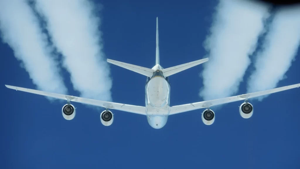
DC-8 in flight. Credit: NASA/SSAI Edward Winstead

 

Let’s say we want to predict the noise that the exhaust of a jet engine is going to produce. What would we need to do? Well, first let’s get out of the way that the geometry of a real jet engine exhaust is complex; we have multiple streams, we have pylons, we have a nearby wing, we have temperature gradients, we have all kinds of complexity we don’t want to deal with.

 

Schematic of a turbofan. Credit: NASA

 

This problem is hard enough, so let’s just start with assuming our exhaust is a single high-speed jet, leaving the engine at a uniform temperature. What does that look like?

Well, this doesn’t exactly look simpler!

Before we get into talking about how the sound is produced, let’s talk about how we measure and quantify the sound itself. We’re interested in understanding how a given input (the jet) produces a given output (the sound), but we need to know what we mean by the output first. The jet we’re looking at above might produce an acoustic spectrum that looks something like this:

We will add a nice clean acoustic spectra here to talk about the sound.

What does this mean? What do the axes represent, and what are the units? How do we measure this, and how do we scale the data appropriately? To answer these questions, click on the acoustics link below, then return here when ready.

 

An introduction to acoustic data

 

What we’re looking at here is an unheated, laboratory scale supersonic jet from a simple round converging nozzle, and it’s still horrendously complex. We need to be able to predict what’s happening outside the jet, what it sounds like far far away, based on all this complexity happening inside and around the jet. We’ve got sound waves going this way, we’ve got sound waves going that way, we’ve got turbulence, we’ve got shocks, we’ve got coherent structures. This still feels like an impossible problem. So let’s break it down step by step.

 

Let’s slow our jet right down. Instead of a supersonic jet, let’s consider a jet going at just a few meters per second.

 

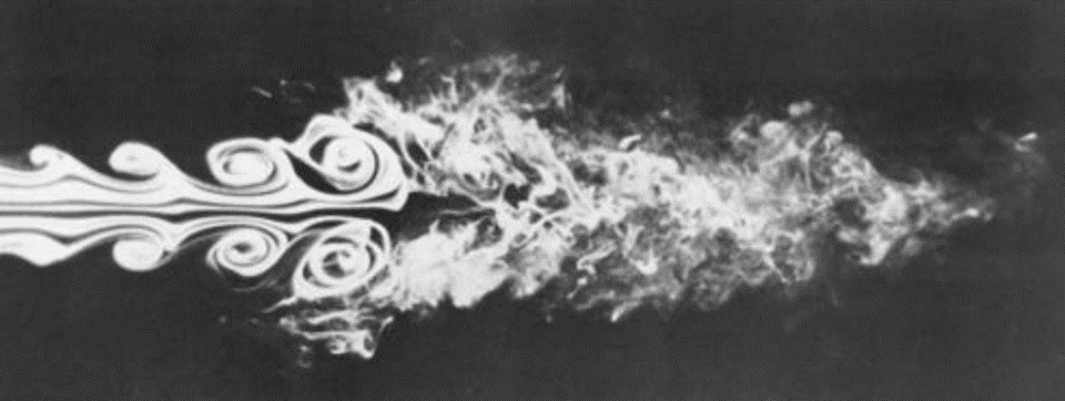
An initially laminar jet transitioning to turbulence via the Kelvin-Helmholtz instability. Credit: An Album of Fluid Motion, The Parabolic Press, 1982.

This jet is now starting out in what we would call the laminar regime; adjacent fluid pathlines do not cross, there is minimal mixing except through diffusion. A laminar flow like this one is extremely quiet, but to keep it laminar, we’d also have to keep it very slow, so that’s not helpful. But this is a good place to start our discussion of jets.

 

When we keep the jet this slow, it seems to have almost nothing in common with that supersonic turbulent jet we saw a moment ago. But if we increase the speed just a little, we see something fairly drastic happen. (Note that this image is a placeholder and will be replaced with our own videos where we vary the speed to induce visible KH instabilities then transition)

 

While the flow starts out parallel, we see these waves developing at the boundaries of the jet, which grow as we move downstream, eventually turning into large vortices.

 

What we are seeing here is known as the Kelvin-Helmholtz instability, which takes us to our first jumping off point: the link below will take you to an overview of the KH instability for jets, what it means and how to calculate it.

 

An introduction to linear stability analysis for shear flows

 

Now that we know a bit more about how the Kelvin-Helmholtz instability works, let’s return to our jet. The KH instability is going to be really important to us for two reasons. One of them we’ll come back to later, but the classical reason is, that this is the mechanism by which our laminar flow becomes turbulent; if we speed up our jet a little more, we can observe this happening.

 

An initially laminar jet transitioning to turbulence via the Kelvin-Helmholtz instability. Credit: An Album of Fluid Motion, The Parabolic Press, 1982.

Turbulence is an incredibly complex topic, and critically important to our understanding of jets, so this takes us to our next jumping off point. Click the link below to jump to the turbulence topic, then return here when ready.

A brief introduction to turbulence

 

So, we have had a brief introduction to the broad topic of turbulence. What does that mean for a turbulent jet, specifically? Due to its nature, we tend to describe turbulence statistically, and we often take the same approach when describing the field of a turbulent jet. We can define the spatial development of a turbulent jet based on these statistical properties, and divide it into several regions based on these definitions.

 

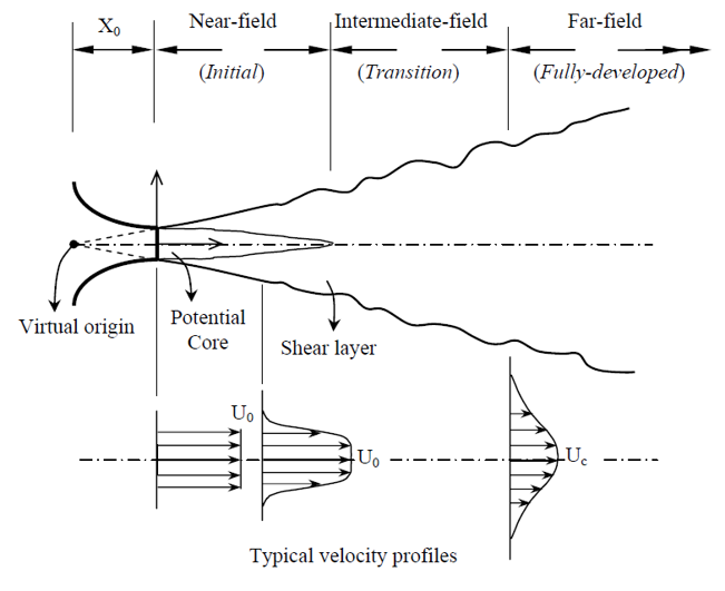
Schematic of a turbulent jet. Taken from Abdel-Rahman, 2010 “A Review of Effects of Initial and Boundary Conditions on Turbulent Jets, WSEAS Transactions on Fluid Mechanics.

 

For a more detailed discussion, refer click on the link below to read a discussion about turbulent jets, then return here.

 

An introduction to turbulent jets

 

So what do we know so far?

The jet comes out of the nozzle, the Kelvin-Helmholtz instability drives a transition to turbulence, and then we can predict something about the shape of the turbulent jet that will result, at least in the mean. But what does this have to do with sound?

Well, let’s look at a jet at a Mach number of 0.9, and for this purpose we’re going to look at a beautiful numerical simulation that has become one of the canonical reference cases for jet noise. This is a a Large-Eddy Simulation of a turbulent jet by Guillaume Bres and colleagues, and it is actually publicly available for download as part of the collection Towne, A., Dawson, S. T., Brès, G. A., Lozano-Durán, A., Saxton-Fox, T., Parthasarathy, A., … & Taira, K. (2023). A database for reduced-complexity modeling of fluid flows. AIAA Journal, 1-26.

We have an incredibly complicated flow field, and we have an incredibly complicated sound field that it is producing. So, how does turbulence produce sound? That is a complicated question, but one that we do have ways of answering. It’s going to take some time and explanation and quite a bit of math though, so click on the link to the “Acoustic Analogies” topic below, then return here when you are ready.

 

An introduction to acoustic analogies

 

We have an exact mathematical framework that tells us how sound can arise from turbulent motions in a fluid flow. We can take a numerical database like this one, calculate the source terms, and predict the sound the flow will produce. This is not particularly useful on its own however, because if we can produce a simulation that gives us all the information we need to build a source model without any simplifications, we can also just measure the sound directly from the simulation. And while the simulation might tell us what the sound is, it doesn’t tell us what is and is not important in the flow when it comes to generating that sound.

Let’s look at this numerical simulation again (I will be making my own animations here, just go with it for now); when we look at a slice side on like this, both the jet and the sound field it produces look pretty chaotic. If we look at the jet end-on though, we see a very different picture. The jet itself still looks chaotic, but the sound field starts to look rather organized and regular.

Is there order in the chaos? Well of course, the answer is yes, but getting at it is going to be tricky. The first way we might try to identify the ordered structures in this system, is through a frequency or wavenumber based decomposition. To do that, we’ll need to understand the use of Fourier transforms. So head over to the section on Fourier Decomposition, and then return here to see what we can do with it.

 

An Introduction to Fourier Transforms

 

So, a decomposition in azimuth gives us a really nice representation of the acoustic field, but a very poor one of the jet itself; a couple of azimuthal modes does not make a good low-rank description of the jet.

Why is the sound field so ordered, while the jet itself seems so chaotic?

 

Well, we’re on our way to answering that, and that’s where we will really get to the heart of the matter, but first let’s add a better tool to our toolkit for trying to find some order in the jet itself; if it’s producing this ordered sound field, there must be some underlying order…

We have used a frequency based decomposition, our Fourier transform, let us now consider other ways we might decompose the flow, specifically an energy based decomposition. Click the link below to jump to the modal decomposition topic, then return here when finished.

 

An introduction to modal decompositions

 

So, what happens if we apply some of these new tools to the simulation data we’ve looked at above? We do indeed, find some order in the chaos; though this jet is highly turbulent, hidden inside that turbulence are structures that actually look very much like those vortices we saw growing in the shear layer of the laminar jet. This brings us now to perhaps the most important thing in our modern understanding of jet noise; even in highly turbulent jets, there are coherent structures within the jet. These coherent structures are in fact produced by the same mechanism that drives transition from laminar to turbulent flow in low Reynolds-number jets; the Kelvin-Helmholtz instability. These structures comprise a relatively small amount of the total turbulent kinetic energy of the jet, but actually produce the vast majority of the sound. This set of facts, taken together, forms what is generally known as the wavepacket framework of jet noise, and it is the lens through which most of our current advances in jet noise has taken place. Click the link below to learn more about it.

 

The wavepacket framework for jet noise

 

So, now we know a lot more about how jets produce sound, and we’ve developed a lot of tools to help us predict this sound, where to next? Well, let’s go back to our original laboratory scale jet that we considered:

There’s more going on here than just turbulence and coherent structures, this is an underexpanded supersonic jet, with a series of shock and expansion cells emanating from the nozzle lip. To learn more about these and how they form, let’s take a brief detour into gas dynamics and compressible flow.

 

Waves in Compressible Flow

 

What does it mean for jet noise to have these shocks in the flow? Well, let’s look again at the sound this supersonic jet is producing in a little more detail. There are actually several distinct mechanisms at work in a shock-containing jet like this one. It’s easiest if we compare the spectrum to that produced by a subsonic jet.

 

Subsonic jet spectra here.

Now, the same supersonic jet spectrum from before.

Supersonic spectra.

 

Aside from the fact the supersonic jet is much louder, the spectra also has a different shape; we see a distinct “hump”, and we see a series of peaks. The hump arises from a phenomenon called “broadband shock-associated noise”, while the peaks arise from a phenomenon called “screech”. Screech is a form of aeroacoustic resonance in jets; click the link below to jump out to a separate discussion on resonance if you are interested, then return here.

 

Aeroacoustic resonance in jets

 

While the jet we’ve been looking at here is supersonic, it’s still quite far from the exhaust of a real jet, as we are not adding any heat to it. Not only is it not hot, the fact it is expanding means that the jet is much colder than the surrounding air, making it quite different to the exhaust of a real engine. When our jet is both hot and supersonic, the wavepackets in the jet move much faster than the ambient speed of sound. This can produce a new source of noise known as “crackle”. To learn more about crackle and associated phenomena, check out the page on non-linear acoustics.

An introduction to non-linear acoustics

 

Is that everything? Well, not quite. In recent years we’ve increasingly understood that while the KH wavepacket is the most important coherent structure in jet noise, it’s not the only one. We know that the state of the boundary layer inside the nozzle actually can play a major role in jet noise, at least for laboratory scale jets (see for instance Bres et al 2018).

 

An introduction to Resolvent Analysis