An Introduction to Acoustic Data

There are of course a great many extant resources available to any student interested in learning about acoustics. This page is not intended as a replacement for these, but rather as a quick introduction for students trying to get up to speed with aeroacoustics in jets and similar flows. For an excellent introductory overview of acoustic waves, the University of Southampton ISVR hosts an outstanding free resource:

ISVR Teaching Material on Waves and Acoustics

Sound is the propagation of a longitudinal wave of pressure and displacement through a compressible medium. The speed at which this disturbance travels is the “speed of sound” for that media. It is only the fluctuations in pressure ( $p'$ that we are able to hear and thus perceive as “sound”, the time-averaged pressure $\bar{p}$ makes no contribution.

$p=\bar{p}+p'$

If we are far away from the flow that is producing the sound, in air that is otherwise not moving, we can likely assume that all fluctuations in pressure arise from acoustic waves. Within the flow itself though, this is not the case; pressure fluctuations are also caused by the bulk motion of fluid and other sources. In fact, within a flow, pressure fluctuations due to acoustic waves often comprise only a tiny fraction of the total pressure fluctuation. One of the classical methods of decomposing fluctuations is to sort them into hydrodynamic, acoustic, and entropic modes, though doing this is not straightforward. Consider including a section on methods to do this here.

When we talk about thermofluid quantities like pressure and temperature, we are used to thinking of them on a linear scale. The pressure fluctuations that we are capable of perceiving as sound (before reaching the level where permanent damage sets in) spans more than ten orders of magnitude. For this reason, we typically represent sound pressure on a logarithmic scale, specifically the decibel (dB) scale. We define Sound Pressure Level (SPL) as:

$SPL (dB \quad re \quad 20 \mu Pa ) = 20 log_{10}(p'_{rms}/p_{ref})$

Here $p_{ref}$ is the reference pressure of $20 \mu Pa$ , and thus formally the units should be written as $dB \quad re \quad 20 \mu Pa$ , though this is frequently not done in the jet noise community. $p'_{rms}$ is the root-mean-square of the fluctuating pressure.

So, how do we measure $p'_{rms}$ ? If we have a numerical simulation, then we simply extract the data at the point we are interested in and proceed with our analysis. If we are constrained to working in the real world, we will need some way of measuring it. Though there are some arcane optical measurements that can extract this quantity in the overwhelming majority of cases, one would simply use a microphone. To learn more about microphones, click below, then return here when finished.

An introduction to microphones.

Once we have acquired our raw pressure data, whether it is from a simulation or from a microphone, we need to process it; the raw pressure information is not particularly useful. There are a few quantities that we might be interested in. One is the “Overall Sound Pressure Level” (OASPL), which is a representation of the total sound pressure across all frequencies, and is measured in decibels. The human ear, however, does not perceive all frequencies with the same intensity, and we are often more interested in working out what the sound pressure level at each individual frequency is, and for this we need some additional signal processing tools. The most fundamental of these is the Fourier Transform, which allows us to decompose our signal on the basis of how much energy exists at each frequency. Follow the link below if you would like more details.

An Introduction to Fourier Transforms

So, we have our core tool to extract the frequency content of signals, in the form of the Fourier Transform. Numerically, this is most-often implemented in the form of the Fast-Fourier Transform, which in Matlab or Python can simply be called via fft(). So, let’s take a recording from a microphone in our laboratory, the raw signal from which looks something like the image below. This recording is sampled at 200kHz (though the microphone cannot really resolve anything above 80kHz, more on that later), so even over a recording period of 0.2s, the signal just looks like a mess. The second image is a zoomed-in representation of the little red box on the left image. This is our raw signal.

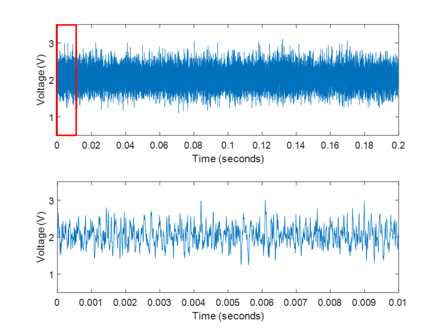
Given what we now know about Fourier Transforms, let’s take our microphone data, in the form of a matrix of [Voltage ; Time], and plug the voltage data straight into our Fast-Fourier Transform, and figure out what frequencies are in this signal!

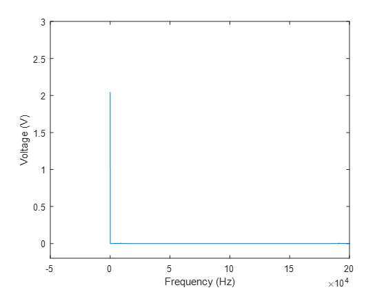
Well, that’s not a very interesting result. If you’re trying this yourself, before you even got to this result, you might have received error messages when you tried to plot a complex number; the Fourier transform contains information about both amplitude and phase, and what is plotted here is the amplitude of the complex number output from the FFT. So what’s going on here? If we look at our original voltage signal, it is based on fluctuations around a DC component of about 2V, and this constant 2V is both always there, and of high amplitude relative to the fluctuations. So when we decompose our signal based on how much energy each frequency contains, our FFT is telling us that the overwhelming majority of the energy is the 2V in the zero-frequency component, aka the DC component, or the time-averaged component. We also know that the time-averaged pressure doesn’t contribute to sound, so removing this from the signal is a fairly obvious first step. Let’s subtract the mean ( $V' = V-\bar{V}$ and try again.

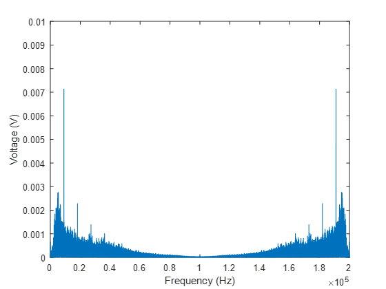
Well, we’ve removed the component at zero frequency, which now means we can actually see the rest of the signal (which was always there, just orders-of-magnitude smaller), but this still doesn’t look like anything resembling the acoustic spectra we started with. What’s going on here? Why is this spectrum symmetric about 100kHz? Well, the Fast-Fourier Transform we are using is simply a particular algorithm for calculating the Discrete-Fourier Transform, and the DFT is periodic. What we are seeing here is the periodicity in the solution. However, Matlab’s conventions for representing this have been a source of pain and confusion for many students (and more senior researchers besides). The output of the DFT should actually be across positive and negative frequencies, and mirrored about zero, whereas the default output from Matlab mirrors the output about $f_s/2$ , where $f_s$ is the sampling frequency. The fftshift command is needed to shift the spectrum such that it is correctly represented, as below:

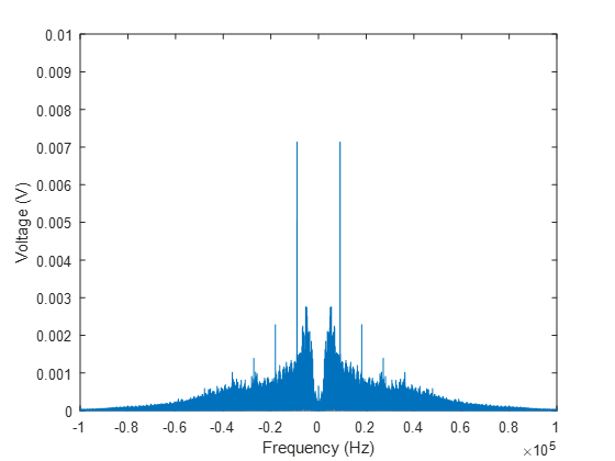
The concept of “negative frequency” is an extremely unintuitive one, and when we’re talking about taking the Fourier transform of a real-valued signal (such as the time-voltage input here), it has little physical meaning. The spectrum in the negative frequencies is simply the complex conjugate of the spectrum in the positive frequencies, and for the purpose of calculating acoustic spectra, we will take advantage of this fact to drop “negative” frequencies from our consideration altogether.

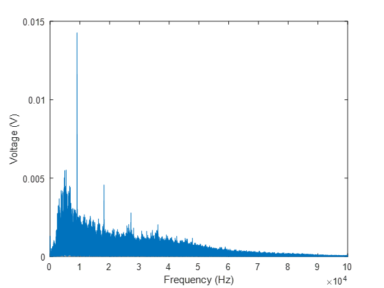
Well, now we finally have something that sort of starts to resemble the spectrum we were looking for; we have a clear peak that might be like the one we saw originally, but it still doesn’t look all that close. Let’s try plotting the Y-axis on a logarithmic scale, and see if that helps.

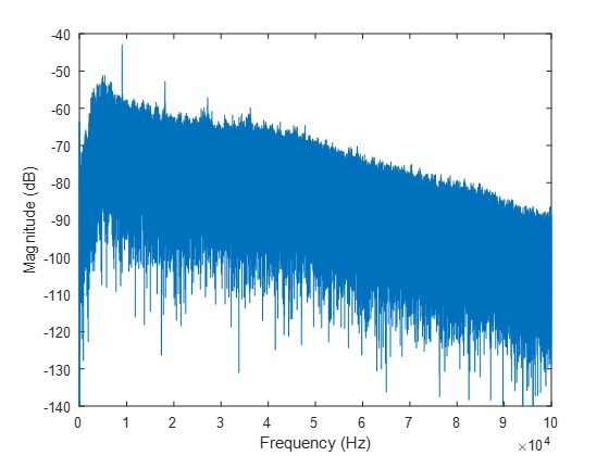
The basic shape is starting to be there, but why is it such a mess? Well, the variance at each frequency is extremely high, which is a consequence of using a Discrete Fourier Transform on a noisy signal. If we are trying to calculate the Power Spectral Density (PSD) $\hat{P}(f)$ as using the DFT, this can be written as:

$\hat{P}(f)=\frac{1}{N} | \sum_{n=0}^{N-1} x [n] e^{-i 2 \pi f n}| ^2$

Todd & Cruz (1996) provide an interesting lens through which to view this, arguing that the PSD can be written in terms of a filter function $h$ :

$\hat{P}(f)=N | \sum_{n=0}^{N-1} h [-k] x [-k]|^2$

where

$h [k]= \frac{1}{N} e^{-i 2 \pi f k}$ $k = -(N-1),...,0$

they go on to state that this final expression is the impulse response of a bandpass filter centered around f. For those of us who are not well-versed in Digital-Signal Processing, the implications of this are not at all clear, but Todd & Cruz elaborate further “So the spectral estimate turns out to be, basically, a single sample of the output of a bandpass filter centered at f. Since only one sample of the output goes into the computation of the estimate, there is no opportunity for averaging to lower the variance of the estimate.”

This then, is the core of the issue, and something that has been recognized since the early days of DSP; adding more samples to the signal on which you are performing a DFT does not reduce the variance! There have been many approaches suggested to address this deficiency in the DSP literature through the years, which are far beyond the scope of our discussion. Rather, we will simply adopt the widely used “Welch’s method”, whereby instead of performing a DFT on the entire dataset, we divide the dataset into separate blocks, calculate the PSD for each, and then calculate an ensemble average to reduce the variance.

So now, rather than applying the FFT to our entire signal of 1E6 samples, we will divide it into 487 blocks, each of 4096 samples, with a 50% overlap in time between each block. The reduction in variance is $\frac{1}{N_{blocks}}$ , so we expect to see a drastically different signal.

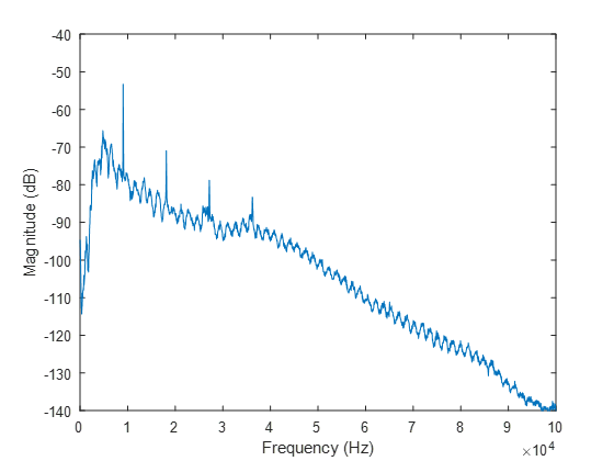
It turns out reducing the variance by almost five-hundred-fold significantly improves your result! We now have something that looks like that first jet-noise spectrum we were trying to reach, but we still have a few more steps to go. Firstly, what is going on with the units on the y-axis? Do we really have negative fifty decibels of sound? Jet noise hardly seems like a problem if this is how loud a supersonic jet is…

Well, let’s think about what our actual input signal was: a voltage reading from the microphone. To produce the logarithmic dB scale, all I have done here is use the mag2db function, which is essentially calculating our magnitude as $y=20log_{10}\frac{V}{1}$ . What does that have to do with sound? Well, without knowing the relationship between the voltage output of the microphone and the pressure it is measuring, the answer is “not much”. We need a calibration factor. We’ll come back to that in a moment.

The second issue we have here, is why do we have this oscillation in our signal amplitude as a function of frequency? There was nothing like this in the original spectrum we saw. What we are actually seeing here is evidence of a flaw in the experiment itself. The data we have been using is from a set Jayson Beekman took in the early stages of trying to configure a new facility, when we were still ironing out issues in the physical setup. What we are seeing in this signal is the signature of constructive and destructive interference, due to the reflection of acoustic waves off hard surfaces. We try to have as much of our facility covered in acoustic foam as possible, but even missing just one spot can be highly detrimental to the measurement, as seen in our result here. This isn’t the kind of issue you want to fix with signal processing; you need to get back in the lab, and fix the experiment. So with that, our final jumping-off point:

Setting Up and Scaling Acoustic Measurements

Let’s compare our spectra above to one taken once we had finished applying all the necessary acoustic treatment to the facility, and now with our signal calibrated appropriately:

Picture here.

We have a clean measurement, and a properly calibrated vertical axis on our graph, with meaningful units. The very final step is to non-dimensionalize our frequency. Dimensional units should only be used with good cause and specific reasons in science, particularly in a field like jet noise. The purpose of our work is to understand the fundamental mechanisms by which jet engines produce noise that impacts the community; these engines are much larger than anything we can operate in the laboratory. Given that the frequencies associated with jet noise depend on the diameter of the jet, talking about a noise peak at 9kHz has no real relevance to either the aviation community, or to anyone whose laboratory facilities are even slightly different to ours. We thus express our frequencies in terms of the Strouhal Number, a non-dimensional value that accounts for both the scale and velocity of the jet. While two different jet facilities will produce jets with very different peak frequencies, in dimensional terms, if they share broadly similar characteristics, they should produce the same peak Strouhal numbers.

With that, our detour discussion into acoustic data comes to an end. Return to the main course by clicking the link below.

ISVR Teaching Material on Waves and Acoustics

An introduction to microphones.

An Introduction to Fourier Transforms

Setting Up and Scaling Acoustic Measurements

Take me back to the main story