Having considered the analytical solution for a planar, incompressible vortex sheet, we now add one additional step of complexity to the problem. Rather than assuming an infinitely thin layer of vorticity separating the two flows, we will now consider a more realistic velocity profile, where the action of viscosity serves to smear the interface into a continuous, rather than discontinuous, variation in velocity.

Image goes here.

Our task is now to consider the stability of this very simple system. For our purposes here, we will consider the most basic possible analysis, which is to assume that the fluid is both inviscid and incompressible. The analysis we are going to conduct, is to consider the equations of motion that describe this system, we will then linearize the system, and consider the response of this linear system to infinitely small perturbations; if the system grows in response to an infinitely small perturbation, it is unstable. To determine if this system is stable, we will undertake the following steps:

Establish the equations of motion.
Linearize these equations of motion.
Propose an ansatz (a model solution) and substitute it into our linearized equations
Obtain an ordinary differential equation from re-arranging our linearized equations
Impose appropriate boundary conditions to reframe the problem as an eigenvalue problem
Solve the eigenvalue problem to determine the stability of the system

To signpost what we’ll be doing, here it is represented diagramatically.

Establish the equations of motion.

We follow the same initial process as when considering the vortex-sheet approximation, beginning with the governing equations. However, we will now include the effects of viscosity in the momentum equation. We will also put the equations in a non-dimensional form:

Put an explanation of the non-dimensionalization step here.

Conservation of Mass in Vector Form (2D, Incompressible)

$\centering \nabla \cdot\mathbf{u} = 0$

Expand to see in non-vector form

$\centering \frac {\partial u} {\partial x} + \frac{\partial v}{\partial y} = 0$

Conservation of X-Momentum in Vector Form (2D, Incompressible)

$\centering \frac{\partial u}{\partial t}+\nabla u \cdot \mathbf{u} +\frac{\partial p}{\partial x} = \frac{1}{Re}\nabla^2 u$

Expand to see in non-vector form

$\centering \frac{\partial u}{\partial t}+ u \frac{\partial u}{\partial x} + v \frac{\partial u}{\partial y} + \frac{\partial p}{\partial x} = \frac{\partial^2 u}{dx^2}+\frac{\partial^2 u}{dy^2}$

Conservation of Y-Momentum in Vector Form (2D, Incompressible)

$\centering \frac{\partial v}{\partial t}+\nabla v \cdot \mathbf{u} + \frac{\partial p}{\partial y} = \frac{1}{Re}\nabla^2 v$

Expand to see in non-vector form

$\centering \frac{\partial v}{\partial t}+ u\frac{\partial v}{\partial x} + v \frac{\partial v}{\partial y} + \frac{\partial p}{\partial x} = \frac{\partial^2 v}{dx^2}+\frac{\partial^2 v}{dy^2}$

Here $u$ and $v$ are our velocity components in the $x$ and $y$ direction, and $\mathbf{u}$ is a vector of these velocities $\mathbf{u}=[u,v]$ .

And that’s it, these are our equations of motion!

Linearize the equations of motion.

As a first step towards linearization, we now apply the Reynolds Decomposition to these equations, meaning we decompose all variables ( $q=[u,v,p]$ ) into a temporal mean $\bar{q}$ and fluctuating $q'$ component.

$\begin{equation*} q=\bar{q}+q' \end{equation*}$

Here we arrive at the first key difference between our approach here and the vortex-sheet approximation; our mean velocity now is some function of our transverse co-ordinate y

$\begin{equation*} \mathbf{u} = \bar{\mathbf{u}}(y)+\mathbf{u}'(x,y,t) \end{equation*}$

Substituting this definition into our continuity equation:

Conservation of Mass – Reynolds Decomposition

$\begin{equation*} \nabla \cdot \mathbf{u} = 0 \nonumber \end{equation*}$

See details of substitution

This step is identical to that performed in the vortex sheet derivation:

$\begin{equation*} \frac{\partial \bar{u}}{\partial x}+\frac{\partial u'}{\partial x}+\frac{\partial \bar{v}}{\partial y}+\frac{\partial v'}{\partial y} = 0 \\ \nonumber \end{equation*}$

Now, to simplify this further, we consider our initial problem description, which is that our flow is “infinitely parallel”, i.e. homogenous in the x direction (and in time).

For the flow to be homogenous in the x direction, there can be no transverse (v) component of velocity in the mean; this transverse component would represent fluid entering or leaving the shear layer, which would result in it growing or shrinking with increasing distance, violating the underpinning assumption. So $\frac{\partial \bar{v}}{\partial y}=0$ .
Since the flow is homogenous in x, $\frac{\partial \bar{u}}{\partial x}=0$

Thus our equation reduces to:

$\centering \boxed{\frac {\partial u'} {\partial x} + \frac{\partial v'}{\partial y} = 0}$

Conservation of x-momentum – Reynolds Decomposition

We now apply the same decomposition to the x-momentum equation.

$\begin{equation*} \[ \centering \frac{\partial u}{\partial t}+\nabla u \cdot \mathbf{u} +\frac{\partial p}{\partial x} = \frac{1}{Re}\nabla^2 u \] \end{equation*}$

Becomes:

$\begin{eqnarray*} \frac{\partial \bar{u}}{\partial t}+\frac{\partial u'}{\partial t} +\bar{u}\frac{\partial{\bar{u}}}{\partial x}+\bar{u}\frac{\partial{u'}}{\partial x}+u'\frac{\partial{\bar{u}}}{\partial x}+u'\frac{\partial{u'}}{\partial x} +{ \bar{v}\frac{\partial{\bar{u}}}{\partial y} +\bar{v}\frac{\partial{u'}}{\partial y}+v'\frac{\partial{\bar{u}}}{\partial y}+v'\frac{\partial{u'}}{\partial y} + \frac{\partial\bar{p}}{\partial x}+\frac{\partial p'}{\partial x} \\=\frac{1}{Re}\nabla^2 \bar{u} + \frac{1}{Re}\nabla^2 {u'} \end{eqnarray*}$

That’s a long one. We can cross out most of these terms however:

See details of terms being crossed out

If we are formulating this problem rigorously, we are considering a base flow that is laminar, which means we are linearizing around a time-invariant solution of the original governing equations:

$\begin{equation*} \[ \centering \frac{\partial \bar{u}}{\partial t}+\nabla \bar{u} \cdot \mathbf{\bar{u}} +\frac{\partial \bar{p}}{\partial x} = \frac{1}{Re}\nabla^2 \bar{u} \] \end{equation*}$

We can thus subtract this solution from our Reynolds-decomposed form of the equations:

$\begin{eqnarray*} \textcolor{red} {\frac{\partial \bar{u}}{\partial t}}+\frac{\partial u'}{\partial t} +\textcolor{red}{ \bar{u}\frac{\partial{\bar{u}}}{\partial x}} +\bar{u}\frac{\partial{u'}}{\partial x}+{u'\frac{\partial{\bar{u}}}{\partial x}}+u'\frac{\partial{u'}}{\partial x} +\textcolor{red}{\bar{v}\frac{\partial{\bar{u}}}{\partial y}} +\bar{v}\frac{\partial{u'}}{\partial y}+v'\frac{\partial{\bar{u}}}{\partial y}+v'\frac{\partial{u'}}{\partial y} +\textcolor{red} { \frac{\partial \bar{p}}{\partial x}}+\frac{\partial p'}{\partial x} \\\ =\textcolor{red}{\frac{1}{Re}\nabla^2 \bar{u}} + \frac{1}{Re}\nabla^2 {u'} \end{eqnarray*}$

Removing the terms in red:

$\begin{equation*} \frac{\partial u'}{\partial t} +\bar{u}\frac{\partial{u'}}{\partial x}+u'\frac{\partial{u'}}{\partial x} +\bar{v}\frac{\partial{u'}}{\partial y}+v'\frac{\partial\bar{u}}{\partial y}+v'\frac{\partial{u'}}{\partial y}+\bar{v}\frac{\partial{u'}}{\partial y} +\frac{\partial p'}{\partial x} = \frac{1}{Re}\nabla^2 {u'} \end{equation*}$

We now once again impose linearization, by setting all products of fluctuations to zero

$\begin{equation*} \frac{\partial u'}{\partial t} +\bar{u}\frac{\partial{u'}}{\partial x}+\textcolor{red}{u'\frac{\partial{u'}}{\partial x}} +\bar{v}\frac{\partial{u'}}{\partial y}+v'\frac{\partial{\bar{u}}}{\partial y}+\textcolor{red}{v'\frac{\partial{u'}}{\partial y}} +\frac{\partial p'}{\partial x} = \frac{1}{Re}\nabla^2 {u'} \end{equation*}$

Leaving:

(1) $\begin{equation*} \frac{\partial u'}{\partial t} +\bar{u}\frac{\partial{u'}}{\partial x} +\bar{v}\frac{\partial{u'}}{\partial y}+v'\frac{\partial{\bar{u}}}{\partial y} +\frac{\partial p'}{\partial x} = \frac{1}{Re}\nabla^2 {u'} \end{equation*}$

Finally, as we are considering a parallel base flow, $\bar{v}=0$ , which removes one additional term:

(2) $\begin{equation*} \frac{\partial u'}{\partial t} +\bar{u}\frac{\partial{u'}}{\partial x} +v'\frac{\partial{\bar{u}}}{\partial y} +\frac{\partial p'}{\partial x} = \frac{1}{Re}\nabla^2 {u'} \end{equation*}$

This finishes our linearization of the x-momentum equation:

$\centering \boxed{ \frac{\partial u'}{\partial t} +\bar{u}\frac{\partial{u'}}{\partial x} +v'\frac{\partial{\bar{u}}}{\partial y} +\frac{\partial p'}{\partial x} = \frac{1}{Re}\nabla^2 u'}$

Conservation of y-momentum – Reynolds Decomposition

Following the same steps as the x-momentum decomposition and substitution yields:

$\centering \boxed{\frac{\partial v'}{\partial t}+\bar{u}\frac{\partial{v'}}{\partial x}+\frac{\partial p'}{\partial y}= \frac{1}{Re}\nabla^2 {v'}}$

Linearized Incompressible 2D Equations of Motion

$\frac {\partial u'} {\partial x} + \frac{\partial v'}{\partial y} = 0$

$\frac{\partial u'}{\partial t} +\bar{u}\frac{\partial{u'}}{\partial x} +v'\frac{\partial{\bar{u}}}{\partial y} +\frac{\partial p'}{\partial x} = \frac{1}{Re}\nabla^2 u'$

$\frac{\partial v'}{\partial t}+\bar{u}\frac{\partial{v'}}{\partial x}+\frac{\partial p'}{\partial y}= \frac{1}{Re}\nabla^2 {v'}$

Reduce to a single equation

At this point, we could continue with the same process we followed in deriving the vortex-sheet relation, i.e. proposing an ansatz and formulating an eigenvalue problem. However, unlike the vortex sheet, we can now no longer reach an analytical solution, and instead will need to solve our system numerically. Prior to doing this, it is possible to re-arrange the three equations above into a single equation; when stability was first being studied, without access to computers, it was necessary to do this to make the problem more tractable. We will follow the same process here, though it is not strictly necessary with modern computational resources.

To reduce to a single equation, we need also reduce our number of unknowns. We have three unknowns at present: $u', v', p'$ . We will now perform some mathematical tricks and re-arrangements to remove both $u'$ and $p'$ , leaving us with a single equation. This next part is not necessarily very intuitive, it may be easiest to just think “It’s necessary to do some fancy mathematical manipulation to make the problem simpler”. Luckily for us, these tricks were worked out long before we were born.

We will perform two separate steps on our path to a single equation representation

I. Take the divergence of the linearized momentum equations to remove $u'$ .

II. Take the Laplacian of the transverse momentum (y-momentum) equation to remove $p'$

I. Take the divergence of the linearized momentum equations.

(3) $\begin{equation*} \nabla \cdot (\frac{\partial u'}{\partial t} +\bar{u}\frac{\partial{u'}}{\partial x} +v'\frac{\partial{\bar{u}}}{\partial y} +\frac{\partial p'}{\partial x} - \frac{1}{Re}\nabla^2 u' ) \end{equation*}$

Considering that $\frac{\partial \bar{u}}{\partial x} = 0$ due to the assumption of homogeneity in x, this resolves to:

(4) $\begin{equation*} \frac{\partial^2 u'}{\partial t \partial x} + \bar{u} \frac{\partial^2 u'}{\partial x^2} +\frac{\partial v'}{\partial x} \frac{\partial{\bar{u}}}{\partial y} +\frac{\partial^2 p'}{\partial x} - \frac{1}{Re}\nabla^2 \frac{\partial u'}{\partial x} \end{equation*}$

Similarly:

(5) $\begin{equation*} \nabla \cdot ( \frac{\partial v'}{\partial t}+\bar{u}\frac{\partial{v'}}{\partial x}+\frac{\partial p'}{\partial y} -\frac{1}{Re}\nabla^2 {v'} ) \end{equation*}$

Resolves to:

(6) $\begin{equation*} \frac{\partial^2 v'}{\partial t \partial y} +\frac{\partial \bar{u}}{\partial y} \frac{\partial v'}{\partial x} + \bar{u} \frac{\partial^2 v'}{\partial x \partial y} +\frac{\partial^2 p'}{\partial y} - \frac{1}{Re}\nabla^2 \frac{\partial v'}{\partial y} \end{equation*}$

These can be set equal to each other, and then some like terms collected:

(7) $\begin{equation*} \frac{\partial'}{\partial t} (\frac{\partial u'}{\partial x} + \frac{\partial v'}{\partial y}) + \bar{u} \frac{\partial}{\partial x} (\frac{\partial u'}{\partial x} + \frac{\partial v'}{\partial y}) + 2 \frac{\partial{\bar{u}}}{\partial y} \frac{\partial v'}{\partial x} + \nabla ^2 p' -\frac{1}{Re} \nabla ^2(\frac{\partial u'}{\partial x} + \frac{\partial v'}{\partial y}) \end{equation*}$

At first glance, this may not seem like it has simplified much at all. But let’s bring back our colour encoding:

(8) $\begin{equation*} \frac{\partial'}{\partial t} \textcolor{blue}{(\frac{\partial u'}{\partial x} + \frac{\partial v'}{\partial y})} + \bar{u} \frac{\partial}{\partial x} \textcolor{blue}{(\frac{\partial u'}{\partial x} + \frac{\partial v'}{\partial y})} + 2 \frac{\partial{\bar{u}}}{\partial y} \frac{\partial v'}{\partial x} + \nabla ^2 p' -\frac{1}{Re} \nabla ^2 \textcolor{blue}{(\frac{\partial u'}{\partial x} + \frac{\partial v'}{\partial y})} = 0 \end{equation*}$

This is our linearized conservation of mass equation, which we know equals zero:

$\frac {\partial u'} {\partial x} + \frac{\partial v'}{\partial y} = 0$

Therefore we can massively simplify this expression:

(9) $\begin{equation*} 2 \frac{\partial{\bar{u}}}{\partial y} \frac{\partial v'}{\partial x} + \nabla ^2 p' = 0 \end{equation*}$

This might seem almost unrecognizable, but this is just a compact form of our linearized conservation of momentum in the x and y directions! We have not changed what we are saying about the physics at all, we’ve just used some mathematical tricks to remove the $u'$ component, and condense the two equations into one.

II. Take the Laplacian of the linearized y-momentum equation.

We now undertake our second bit of mathematical trickery, seeking to remove the $p'$ component in the expression, on our journey to reduce this to a single equation. Here, we will take the Laplacian of the linearized y-momentum equation:

$\nabla^2 (\frac{\partial v'}{\partial t}+\bar{u}\frac{\partial{v'}}{\partial x}+\frac{\partial p'}{\partial y} - \frac{1}{Re}\nabla^2 {v'}) = 0$

To do this, we will need to make use of a vector-calculus identity:

$\begin{equation*} \nabla^2 (fg) = f\nabla^2 g+g \nabla^2 f + 2 \frac{\partial f} {\partial x} \frac{\partial g} {\partial x} + 2 \frac{\partial f} {\partial y} \frac{\partial g} {\partial y} \end{equation*}$

$\frac{\partial \nabla^2 v'}{\partial t} +\nabla^2 \bar{u} \frac{\partial v' }{\partial x} + \bar{u} \frac{\partial{\nabla^2 v'}}{\partial x} + 2( \frac{\partial \bar{u}}{\partial x} \frac{\partial^2 v'}{\partial x^2} + \frac{\partial \bar{u}}{\partial y} \frac{\partial^2 v'}{\partial x \partial y}) +\frac{\partial \nabla^2 p'}{\partial y} - \frac{1}{Re}\nabla^4 {v'} = 0$

This might be a pretty scary looking equation, but like many of the steps here, this is only a short stopover on the way to something simple and elegant. We can pull some terms together by considering the convective/material derivative $(\frac{\partial}{\partial t} + \bar{u} \frac{\partial}{\partial x})$ , and by remembering our base flow does not vary in the x-direction, so:

$\nabla^2 \bar{u} = \frac{d^2 \bar{u}}{d y^2}$

Substituting:

$(\frac{\partial}{\partial t} + \bar{u} \frac{\partial}{\partial x}) \nabla^2 v' + \frac{\partial v' }{\partial x} \frac{d^2 \bar{u}}{d y^2} + 2 \frac{\partial \bar{u}}{\partial x} \frac{\partial^2 v'}{\partial x^2} + 2 \frac{\partial \bar{u}}{d y} \frac{\partial^2 v'}{\partial x \partial y} +\frac{\partial \nabla^2 p'}{\partial y} - \frac{1}{Re}\nabla^4 {v'} = 0$

Given our assumption of locally parallel flow, $\partial \bar{u}/\partial x = 0$ , which removes one term

$(\frac{\partial}{\partial t} + \bar{u} \frac{\partial}{\partial x}) \nabla^2 v' + \frac{\partial v' }{\partial x} \frac{d^2 \bar{u}}{d y^2} + 2 \frac{d \bar{u}}{d y} \frac{\partial^2 v'}{\partial x \partial y} +\frac{\partial \nabla^2 p'}{\partial y} - \frac{1}{Re}\nabla^4 {v'} = 0$

We can now take our result from calculating the divergence of the linearized momentum equations:

(10) $\begin{equation*} \nabla ^2 p' = -2 \frac{d \bar{u}}{d y} \frac{\partial v'}{\partial x} \end{equation*}$

and use this to calculate the $\frac{ \partial \nabla ^2 p'}{\partial y}}$ term:

(11) $\begin{equation*} \frac{ \partial \nabla ^2 p'}{\partial y} = -2 \frac{d^2 \bar{u}}{d y^2} \frac{\partial v'}{\partial x} -2 \frac{d \bar{u}}{d y} \frac{\partial^2 v'}{\partial x \partial y} \end{equation*}$

and substitute this into the Laplacian of our linearized y-momentum equation:

$(\frac{\partial}{\partial t} + \bar{u} \frac{\partial}{\partial x}) \nabla^2 v' + \frac{\partial v' }{\partial x} \frac{\partial^2 \bar{u}}{\partial y^2} + 2 \frac{d \bar{u}}{d y} \frac{\partial^2 v'}{\partial x \partial y} -2 \frac{d ^2 \bar{u}}{d y^2} \frac{\partial v'}{\partial x} -2 \frac{d \bar{u}}{d y} \frac{\partial^2 v'}{\partial x \partial y} - \frac{1}{Re}\nabla^4 {v'} = 0$

Our four terms outside the convective derivative on the LHS reduce to one, leaving us with:

$(\frac{\partial}{\partial t} + \bar{u} \frac{\partial}{\partial x}) \nabla^2 v' -\frac{d^2 \bar{u}}{d y^2} \frac{\partial v'}{\partial x} = \frac{1}{Re}\nabla^4 {v'}$

Stop for a moment and consider, that we have reduced a system of three equations and three unknowns to a single equation in terms of a single unknown ( $v'$ ), without removing any of the physics. This expression contains our original physical laws: the conservation of mass, and of momentum in both the x and y directions. We now work towards a numerical solution of this equation.

Propose an ansatz

At this point in the vortex-sheet problem, we imposed a normal-mode ansatz with a post-hoc justification “perturbations look like waves, so let’s assume the solution is wavelike.”

At this stage, we will apply a little more rigour on the mathematical side. Our problem has three dimensions (x,y,t), and two of these are homogenous (x,t) due to the assumptions underpinning our problem; we have assumed a locally parallel flow, which means no variation in x, thus x is a homogenous direction. Our base state is time invariant, thus time can also be taken as homogenous. Given we have two homogenous dimensions, we can represent these dimensions on a Fourier basis; as y is not homogenous, we cannot represent it on a Fourier basis. Thus our normal mode ansatz includes some functional description of our variables in the y-direction, and a Fourier representation of x and t. For our state variables $q'=[u',v',p']$ , our ansatz is:

$\begin{equation*} q'=\hat{q}(y)e^{i(kx-\omega t)} \end{equation*}$

Remembering from our vortex-sheet derivation, key outcomes of assuming a normal-mode ansatz for a linear system are:

Each normal mode satisfies the linear system, and can thus be treated independently – the solutions are independent.
The summation of all the individual normal modes represents the complete motion of the system.

When dealing with stability theory, different texts (and sometimes even the same text in different chapters) will switch between defining the ansatz in terms of frequency $\omega$ or phase speed $c$ , which are linked to wavenumber $k$ by the dispersion relation:

$\begin{equation*} c = \frac{\omega}{k} \end{equation*}$

Here we will use the ansatz in the form:

$\begin{equation*} q'=\hat{q}(y)e^{ik(x-ct)} \end{equation*}$

This is identical to our previous ansatz, just expressed in terms of phase velocity rather than frequency.

Now that we have our linearized equation and our ansatz, the next step is to substitute the ansatz into these linearized equations

Ansatz Substitution

To substitute our ansatz into our single-equation expression of the linearized conservation laws, we need to consider how the various derivative operators act on our ansatz.

$\begin{eqnarray*} \frac{\partial '}{\partial t}=-ikc \\ \nonumber \frac{\partial '}{\partial x}=i k \\ \nonumber \frac{\partial^2 '}{\partial x^2}= -k^2 \\ \nonumber \nabla^2=\frac{d^2}{dy^2} -k^2 \\ \nonumber \nabla^4=\frac{d^4}{dy^4} -2k^2\frac{d^2}{dy^2}+k^4 \\ \nonumber \end{eqnarray*}$

Now it is simply a matter of substituting these terms into our linearized equations of motion.

$(\frac{\partial}{\partial t} + \bar{u} \frac{\partial}{\partial x}) \nabla^2 v' -\frac{d^2 \bar{u}}{dy^2} \frac{\partial v'}{\partial x} = \frac{1}{Re}\nabla^4 {v'}$

Becomes

$(-ikc + \bar{u} ik) [\frac{d^2}{dy^2} -k^2] \hat{v} -ik \frac{d^2 \bar{u}}{d y^2} \hat{v} = \frac{1}{Re} [\frac{d^4}{dy^4} -2k^2\frac{d^2}{dy^2}+k^4] \hat{v}$

Divide both sides by $ik$ , and we have the goal we have been working towards, the Orr-Sommerfeld equation, which rather than being a partial differential equation, is a fourth-order ordinary differential equation:

$(\bar{u}-c) [\frac{d^2}{dy^2} -k^2] \hat{v} - \frac{d^2 \bar{u}}{d y^2} \hat{v} = \frac{1}{ik Re} [\frac{d^4}{dy^4} -2k^2\frac{d^2}{dy^2}+k^4] \hat{v}$

If we take the inviscid limit, setting viscosity to zero by setting the Reynolds number to infinity, we reduce to the Rayleigh equation, a second-order ordinary differential equation:

$(\bar{u}-c) [\frac{d^2}{dy^2} -k^2] \hat{v} - \frac{d^2 \bar{u}}{d y^2} \hat{v} = 0$

Solving the Rayleigh Equation

Unlike our vortex-sheet problem, we cannot produce an analytical solution to either the Rayleigh or Orr-Sommerfeld equations. Instead, we will solve them numerically. To do this, we will turn our ODE into a matrix problem. We will start with the simpler case of the Rayleigh equation, which reduces our problem to second order.

We want to cast our problem in the form:

$Lv=cFv$

Where L and F are blah

To do this we re-arrange our Rayleigh equation such that c appears on the right-hand side:

$(\bar{u} (\frac{d^2}{dy^2} -k^2) - \frac{d^2 \bar{u}}{d y^2} ) \hat{v} = c (\frac{d^2}{dy^2} -k^2) \hat{v}$

We define a differential operator matrix D, and then we can write this as:

$(L_1 + L_2 + L_3)v=c(F_1+F_2)v$

$\begin{eqnarray*} L_1 =\bar{u}D^2 \\ \nonumber L_2 =-\bar{u}k^2 \\ \nonumber L_3 =-D^2\bar{u} \\ \nonumber F_1 = D^2 \\ \nonumber F_2 = -k^2 \\ \nonumber \end{eqnarray*}$

Now our task is to build the matrices that will allow us to solve this as an eigenvalue problem. For our example here, we will use Matlab, though this could just as easily be done in Python.

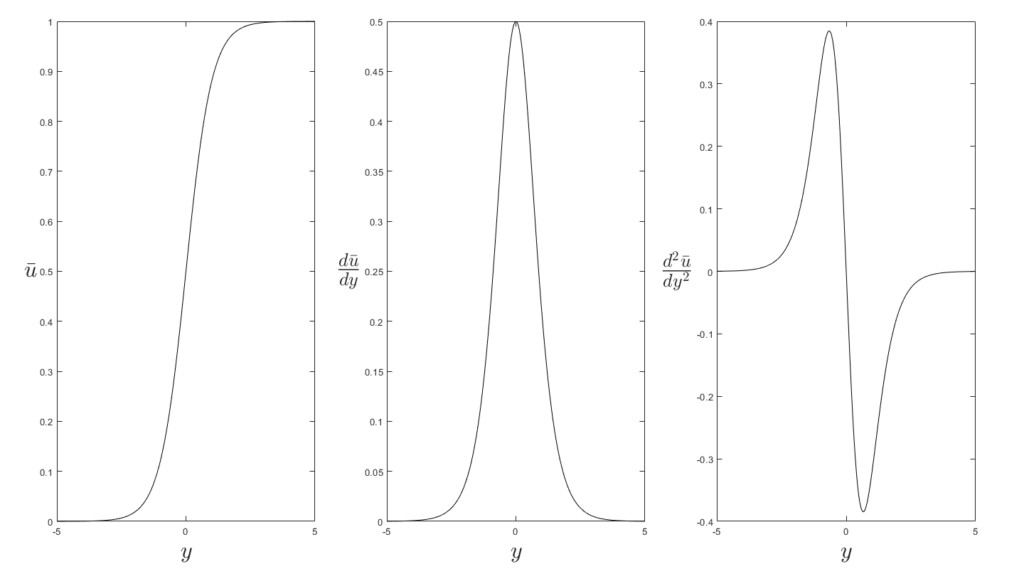
First, let us define the velocity profile whose stability we are considering; these equations require a base flow. Though we have only referenced it obliquely, strictly the Rayleigh equation is only applicable to a laminar solution of the full non-linear Navier-Stokes equations (though we will use it for other things as well). One such solution, is a hyperbolic-tangent function defined as:

$\begin{equation*} \bar{u} = 0.5(1+tanh(y)) \end{equation*}$

Which looks like this:

First we will define the grid over which we will discretise the problem. There are many ways one could discretize a problem like this numerically, with the leading candidates being a classical finite -difference scheme, or what we will use, which is polynomial interpolants. Getting into the “why” is beyond the scope of this course, we will simply state that for many of the problems we consider, polynomial interpolant schemes using Chebyshev Polynomials converge much faster than finite-difference schemes. The reason for this is that the derivative of a Chebyshev polynomial is calculated using information from every point on the grid. Matlab has an inbuilt cheb function which we will use here:

[D,y]=cheb(N)

This defines our grid (y), and its differentiation matrix (D).

We calculate our baseflow as:

u = 0.5*(1+tanh(y))

We then calculate our second-derivative matrix simply as

D2 = D*D;

What are our “differentiation matrices”? They are expressions of the first and second derivatives $d/dy$ $d^2/dy^2$ for the particular grid we have defined on y. To demonstrate this, we calculate the derivatives of our discretised function $u = 0.5*(1+tanh(y))$ , and plot them against the analytical derivatives of our tanh function:

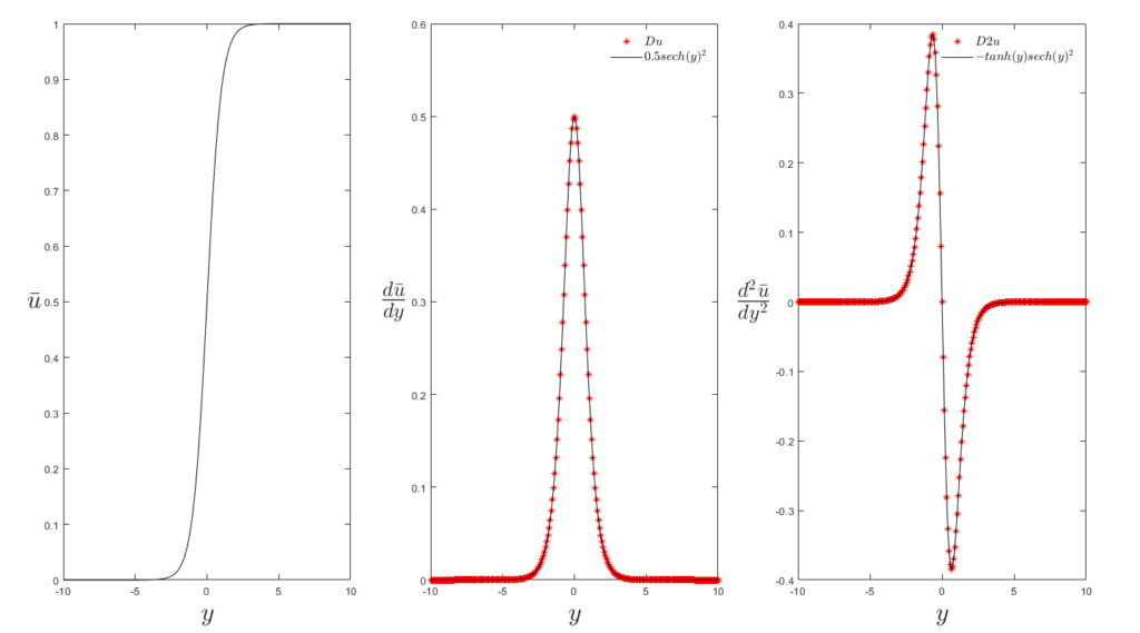
Hopefully this makes it a little more intuitive; our differential matrices D and D2 are a simply a numerical implementation of a derivative calculation.

Now we will construct our matrices L and F. Here we need to consider our linear algebra carefully. We have defined our velocity profile as a column vector of size $u_{N+1,1}$ , while our D2 matrix is a square matrix $D2_{N+1,N+1}$ . If we first consider $L_3 =-D^2\bar{u}$ , we can directly evaluate this. To illustrate, we will reduce it to a 3 x 3 matrix, though any realistic Chebyshev grid will have many more points:

The square matrix operates on the vector of velocities to produce a column vector containing the second derivative of the velocity at each point on the original grid, represented in a column vector of size $(N+1,1)$ .

We now consider $L_2 =-\bar{u}k^2$ . This is a column vector of $u_{N+1,1}$ , multiplied by a single scalar value $k$ , meaning our L2 would come out as a column vector of size $u_{N+1,1}$ . This is the same size as our $L_3$ , so there is no issue there.

However, moving to $L_1 =\bar{u}D^2$ we have to be somewhat more careful. This is the product of an $u_{N+1,1}$ column vector with a square matrix of size $D2_{N+1,N+1}$ . This is not an operation we can perform, so we will need to transform one of our two matrices. We need to preserve the size of our differentiation matrix D2, as it needs to be able to operate on a variable defined on our column vector of size $(N+1,1)$ . What we want is for each row of $D2(i,:)$ to be multiplied by the mean velocity at that grid point $u(i,:)$ . The way to do this is to turn our column vector for $u$ into a diagonal matrix:

U = diag(u);

We can then calculate L1 as:

L1 = U*D2;

Now that our $L_1$ matrix is square, we need our $L_2$ and L_3 $matrices to likewise be square, or else we cannot add them. For$ L_2 $we can simply use the same approach as$ L_1 $; we use our diagonal matrix <em>U</em>, such that: <blockquote>L2 = -U*k^2;</blockquote> <img class="aligncenter wp-image-1111" src="https://daniel.edgington-mitchell.com/wp-content/uploads/2025/04/L2-1024x170.png" alt="" width="540" height="90" /> This leaves us with$ L_3 $, which is currently producing a column vector of size$ (N+1,1) $, containing the values of the second derivative of$ u(y) $at each point on our grid. Using the same justification for diagonalizing the original$ u $matrix, we now do the same for$ d^2u/dy^2$, and diagonalize the output, rather than the input:

L3 = -1*diag(D2*u);

To construct our F matrix, we define F1:

F1 = D^2

F2 is simply a scalar quantity, which needs to be added to a square matrix. The appropriate way to do this is to put the scalar quantity on the diagonal terms, which we can do by multiplying the scalar by the identify matrix, such that:

F2 = -k^2 * eye(size(D2));

If any step of this was unclear, please let me know. The purpose of this section is to be a basic introduction to the material; no question is too basic, no question is “stupid”.

Dr. Daniel Edgington-Mitchell

One step closer to the real Kelvin-Helmholtz problem – Rayleigh and Orr Sommerfeld

Establish the equations of motion.

Put an explanation of the non-dimensionalization step here.

Linearize the equations of motion.

Conservation of Mass – Reynolds Decomposition

Conservation of x-momentum – Reynolds Decomposition

Conservation of y-momentum – Reynolds Decomposition

Linearized Incompressible 2D Equations of Motion

Reduce to a single equation

I. Take the divergence of the linearized momentum equations.

II. Take the Laplacian of the linearized y-momentum equation.

Propose an ansatz

Ansatz Substitution

Solving the Rayleigh Equation

If any step of this was unclear, please let me know. The purpose of this section is to be a basic introduction to the material; no question is too basic, no question is “stupid”.